In-class Exercise 2:

Getting Started

pacman::p_load(tmap,sf,sfdep,tidyverse,knitr, plotly,zoo,kendall)

The Data

Importing the data

• Hunan, a geospatial data set in ESRI shapefile format

• Hunan_2012, an attribute data set in csv format

hunan <- st_read(dsn = "data/geospatial", layer = "Hunan")

Reading layer `Hunan' from data source 
  `/Users/youting/ytquek/ISSS624/In-class Exercise/In-class Exercise 2/data/geospatial' 
  using driver `ESRI Shapefile'
Simple feature collection with 88 features and 7 fields
Geometry type: POLYGON
Dimension:     XY
Bounding box:  xmin: 108.7831 ymin: 24.6342 xmax: 114.2544 ymax: 30.12812
Geodetic CRS:  WGS 84

hunan2012 <- read_csv("data/aspatial/Hunan_2012.csv")

Combine both data frames

hunan_GDPPC <- left_join(hunan,hunan2012) %>%
  select(1:4, 7, 15)

Computing Contiguity Spatial Weights

Use poly2nb() of spdep package to compute contiguity weight matrices for the study area. This function builds a neighbours list based on regions with contiguous boundaries. Note: A “queen” argument taking TRUE/FALSE option can be passed. Default is set to TRUE.

Computing (QUEEN) contiguity based neighbours

wm_q <- hunan_GDPPC %>%
  mutate(nb = st_contiguity(geometry),
         wt = st_weights(nb, style = "W"),
         .before = 1)

Global Spatial Autocorrelation

Compute global spatial autocorrelation statistics and to perform spatial complete randomness test for global spatial autocorrelation.

Computing local Moran’s I

Local Moran’s I of GDPPC at country level

lisa <- wm_q %>%
  mutate(local_moran = local_moran(
    GDPPC, nb, wt, nsim = 99),
    .before = 1) %>%
  unnest(local_moran)

Time Series Cube

GDPPC <- read_csv("data/aspatial/Hunan_GDPPC.csv")

GDPPC_st <- spacetime(GDPPC, hunan, 
                      .loc_col = "County",
                      .time_col = "Year")
is_spacetime_cube(GDPPC)

[1] FALSE

GDPPC_nb <- GDPPC_st %>%
  activate("geometry") %>%
  mutate(nb = include_self(st_contiguity(geometry)),
         wt = st_inverse_distance(nb,geometry,
                                  scale = 1,
                                  alpha=1),
         .before = 1) %>%
  set_nbs("nb") %>%
  set_wts("wt")

Computing Gi*

gi_stars <- GDPPC_nb %>%
  group_by(Year) %>%
  mutate(gi_star = local_gstar_perm(
    GDPPC, nb, wt)) %>%
  tidyr::unnest(gi_star)

Emerging Hot Spots

ehsa <- emerging_hotspot_analysis(
  x = GDPPC_st,
  .var = "GDPPC",
  k = 1,
  nsim = 99
)

hunan_ehsa <- hunan %>%
  left_join(ehsa,
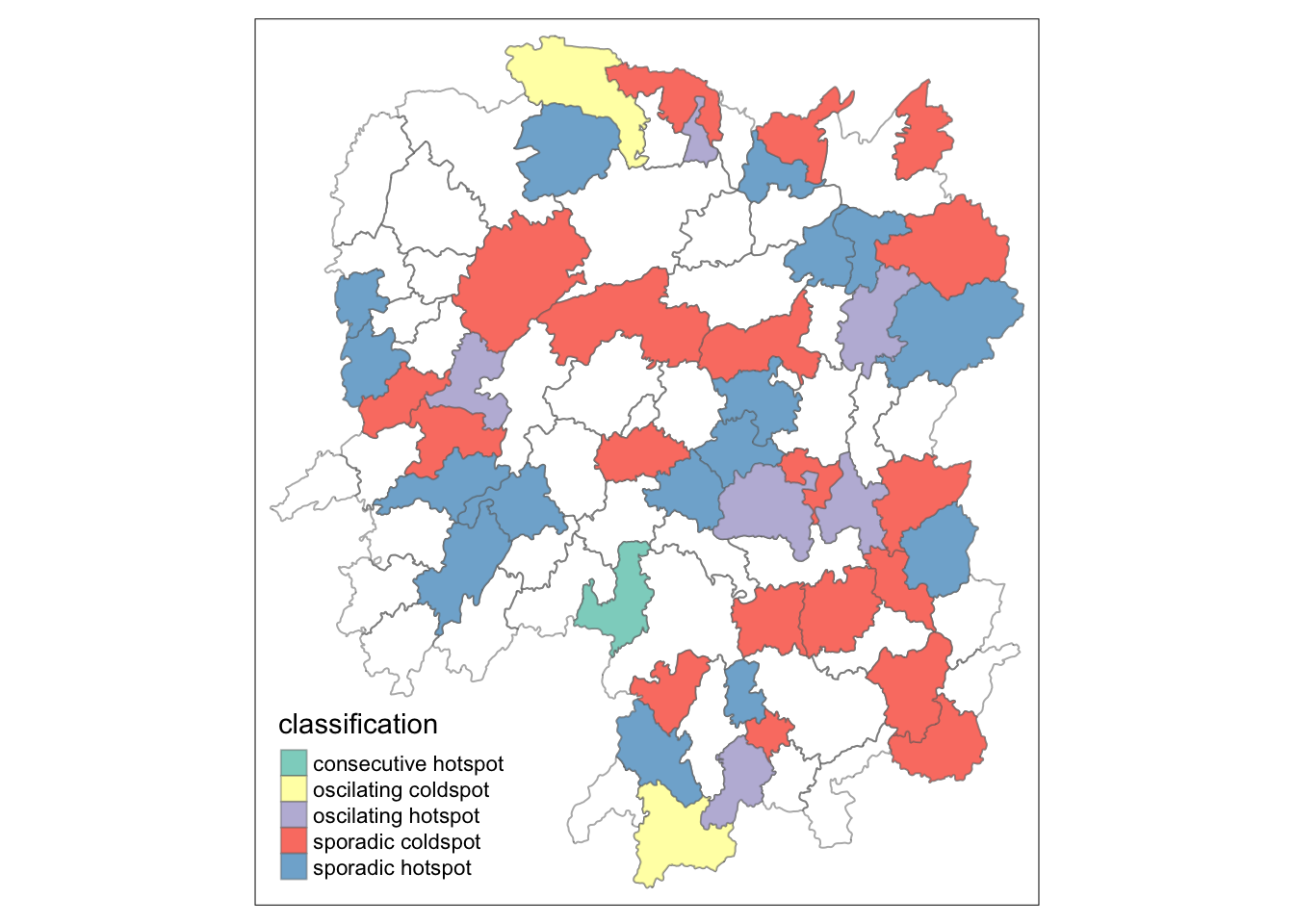
            by = join_by(County==location))

Visualising the distribution of EHSA classes

ehsa_sig <- hunan_ehsa %>%
  filter(p_value < 0.05)

tmap_mode("plot")
tm_shape(hunan_ehsa) +
  tm_polygons +
  tm_borders(alpha = 0.5) +
tm_shape(ehsa_sig) +
  tm_fill("classification") +
  tm_borders(alpha = 0.4)